Kriging

Kriging is a group of geostatistical techniques to interpolate the value of a random field (e.g., the elevation, z, of the landscape as a function of the geographic location) at an unobserved location from observations of its value at nearby locations.

The theory behind interpolation and extrapolation by kriging was developed by the French mathematician Georges Matheron based on the Master's thesis of Daniel Gerhardus Krige, the pioneering plotter of distance-weighted average gold grades at the Witwatersrand reef complex in South Africa. The English verb is to krige and the most common noun is kriging; both are often pronounced with a hard "g", following the pronunciation of the name "Krige".

Interpolation

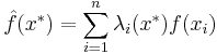
Kriging belongs to the family of linear least squares estimation algorithms. As illustrated in Figure 1, the aim of kriging is to estimate the value of an unknown real-valued function, $f$ , at a point, $x^*$ , given the values of the function at some other points, $x_1,\ldots, x_n$ . A kriging estimator is said to be linear because the predicted value $\hat f(x^*)$ is a linear combination that may be written as

$\hat f(x^*) = \sum_{i=1}^n \lambda_i(x^*) f(x_i)$ .

The weights $\lambda_i(x^*)$ are solutions of a system of linear equations which is obtained by assuming that $f$ is a sample-path of a random process $F(x)$ , and that the error of prediction

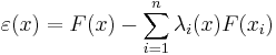
$\varepsilon(x) = F(x) - \sum_{i=1}^n \lambda_i(x) F(x_i)$

is to be minimized in some sense. For instance, the so-called simple kriging assumption is that the mean and the covariance of $F(x)$ is known and then, the kriging predictor is the one that minimizes the variance of the prediction error.

Applications

Although kriging was developed originally for applications in geostatistics, it is a general method of statistical interpolation that can be applied within any discipline to sampled data from random fields that satisfy the appropriate mathematical assumptions.

To date kriging has been used in a variety of disciplines, including the following:

and many others.

Mathematical details

General equations

Kriging interpolates the value $Z(x_0)$ of a random field $Z(x)$ (e.g. the elevation $Z$ of the landscape as a function of the geographic location $x$ ) at an unobserved location $x_0$ from observations $z_i=Z(x_i),\;i=1,\ldots,n$ of the random field at nearby locations $x_1,\ldots,x_n$ . Kriging computes the best linear unbiased estimator $\hat{Z}(x_0)$ of $Z(x_0)$ based on a stochastic model of the spatial dependence quantified either by the variogram $\gamma(x,y)$ or by expectation $\mu(x)=E[Z(x)]$ and the covariance function $c(x,y)$ of the random field.

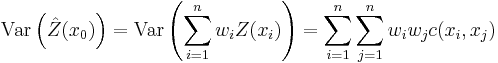
The kriging estimator is given by a linear combination

$\hat{Z}(x_0)=\sum_{i=1}^n w_i(x_0) Z(x_i)$

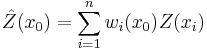
of the observed values $z_i=Z(x_i)$ with weights 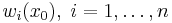$w_i(x_0),\;i=1,\ldots,n$ chosen such that the variance (also called kriging variance or kriging error):

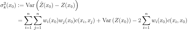
$\begin{align} \sigma^2_k(x_0) &:=\mathrm{Var}\left(\hat{Z}(x_0)-Z(x_0)\right) \\ &=\sum_{i=1}^n\sum_{j=1}^n w_i(x_0) w_j(x_0) c(x_i,x_j) %2B \mathrm{Var}\left(Z(x_0)\right)-2\sum_{i=1}^nw_i(x_0)c(x_i,x_0) \end{align}$

is minimized subject to the unbiasedness condition:

$\mathrm{E}[\hat{Z}(x)-Z(x)]=\sum_{i=1}^n w_i(x_0)\mu(x_i) - \mu(x_0) =0$

The kriging variance must not be confused with the variance

$\mathrm{Var}\left(\hat{Z}(x_0)\right)=\mathrm{Var}\left(\sum_{i=1}^n w_iZ(x_i)\right)=\sum_{i=1}^n\sum_{j=1}^n w_i w_j c(x_i,x_j)$

of the kriging predictor $\hat{Z}(x_0)$ itself.

Methods

Depending on the stochastic properties of the random field different types of kriging apply. The type of kriging determines the linear constraint on the weights $w_i$ implied by the unbiasedness condition; i.e. the linear constraint, and hence the method for calculating the weights, depends upon the type of kriging.

Classical methods of kriging are

Simple kriging assumes a known constant trend: $\mu(x)=0$ .
Ordinary kriging assumes an unknown constant trend: $\mu(x)=\mu$ .
Universal kriging assumes a general polynomial trend model, such as linear trend model $\mu(x)=\sum_{k=0}^p \beta_k f_k(x)$ .
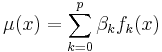IRFk-kriging assumes $\mu(x)$ to be an unknown polynomial in $x$ .
Indicator kriging uses indicator functions instead of the process itself, in order to estimate transition probabilities.
Multiple-indicator kriging is a version of indicator kriging working with a family of indicators. However, MIK has fallen out of favour as an interpolation technique in recent years. This is due to some inherent difficulties related to operation and model validation. Conditional simulation is fast becoming the accepted replacement technique in this case.
Disjunctive kriging is a nonlinear generalisation of kriging.
Lognormal kriging interpolates positive data by means of logarithms.

Simple kriging

Simple kriging is mathematically the simplest, but the least general. It assumes the expectation of the random field to be known, and relies on a covariance function. However, in most applications neither the expectation nor the covariance are known beforehand.

Simple kriging assumptions

The practical assumptions for the application of simple kriging are:

wide sense stationarity of the field.
The expectation is zero everywhere: $\mu(x)=0$ .
Known covariance function $c(x,y)=\mathrm{Cov}(Z(x),Z(y))$

Simple kriging equation

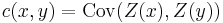
The kriging weights of simple kriging have no unbiasedness condition and are given by the simple kriging equation system:

$\begin{pmatrix}w_1 \\ \vdots \\ w_n \end{pmatrix}= \begin{pmatrix}c(x_1,x_1) & \cdots & c(x_1,x_n) \\ \vdots & \ddots & \vdots \\ c(x_n,x_1) & \cdots & c(x_n,x_n) \end{pmatrix}^{-1} \begin{pmatrix}c(x_1,x_0) \\ \vdots \\ c(x_n,x_0) \end{pmatrix}$

This is analogous to a linear regression of $Z(x_0)$ on the other $z_1 , \ldots, z_n$ .

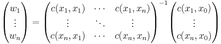
Simple kriging interpolation

The interpolation by simple kriging is given by:

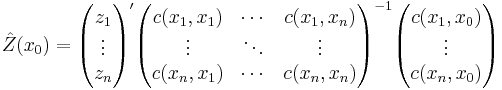
$\hat{Z}(x_0)=\begin{pmatrix}z_1 \\ \vdots \\ z_n \end{pmatrix}' \begin{pmatrix}c(x_1,x_1) & \cdots & c(x_1,x_n) \\ \vdots & \ddots & \vdots \\ c(x_n,x_1) & \cdots & c(x_n,x_n) \end{pmatrix}^{-1} \begin{pmatrix}c(x_1,x_0) \\ \vdots \\ c(x_n,x_0)\end{pmatrix}$

Simple kriging error

The kriging error is given by:

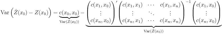
$\mathrm{Var}\left(\hat{Z}(x_0)-Z(x_0)\right)=\underbrace{c(x_0,x_0)}_{\mathrm{Var}(Z(x_0))}- \underbrace{\begin{pmatrix}c(x_1,x_0) \\ \vdots \\ c(x_n,x_0)\end{pmatrix}' \begin{pmatrix} c(x_1,x_1) & \cdots & c(x_1,x_n) \\ \vdots & \ddots & \vdots \\ c(x_n,x_1) & \cdots & c(x_n,x_n) \end{pmatrix}^{-1} \begin{pmatrix}c(x_1,x_0) \\ \vdots \\ c(x_n,x_0) \end{pmatrix}}_{\mathrm{Var}(\hat{Z}(x_0))}$

which leads to the generalised least squares version of the Gauss-Markov theorem (Chiles & Delfiner 1999, p. 159):

$\mathrm{Var}(Z(x_0))=\mathrm{Var}(\hat{Z}(x_0))%2B\mathrm{Var}\left(\hat{Z}(x_0)-Z(x_0)\right).$

Ordinary kriging

Ordinary kriging is the most commonly used type of kriging. It assumes a constant but unknown mean.

Typical ordinary kriging assumptions

The typical assumptions for the practical application of ordinary kriging are:

Intrinsic stationarity or wide sense stationarity of the field
enough observations to estimate the variogram.

The mathematical condition for applicability of ordinary kriging are:

The mean $E[Z(x)]=\mu$ is unknown but constant
The variogram $\gamma(x,y)=E[(Z(x)-Z(y))^2]$ of $Z(x)$ is known.

Ordinary kriging equation

The kriging weights of ordinary kriging fulfill the unbiasedness condition

$\sum_{i=1}^n \lambda_i = 1$

and are given by the ordinary kriging equation system:

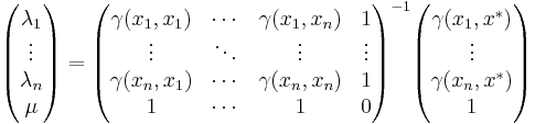
$\begin{pmatrix}\lambda_1 \\ \vdots \\ \lambda_n \\ \mu \end{pmatrix}= \begin{pmatrix}\gamma(x_1,x_1) & \cdots & \gamma(x_1,x_n) &1 \\ \vdots & \ddots & \vdots & \vdots \\ \gamma(x_n,x_1) & \cdots & \gamma(x_n,x_n) & 1 \\ 1 &\cdots& 1 & 0 \end{pmatrix}^{-1} \begin{pmatrix}\gamma(x_1,x^*) \\ \vdots \\ \gamma(x_n,x^*) \\ 1\end{pmatrix}$

the additional parameter $\mu$ is a Lagrange multiplier used in the minimization of the kriging error $\sigma_k^2(x)$ to honor the unbiasedness condition.

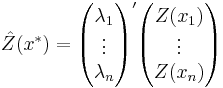
Ordinary kriging interpolation

The interpolation by ordinary kriging is given by:

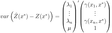
$\hat{Z}(x^*)=\begin{pmatrix}\lambda_1 \\ \vdots \\ \lambda_n \end{pmatrix}' \begin{pmatrix}Z(x_1) \\ \vdots \\ Z(x_n) \end{pmatrix}$

Ordinary kriging error

The kriging error is given by:

$var\left(\hat{Z}(x^*)-Z(x^*)\right)= \begin{pmatrix}\lambda_1 \\ \vdots \\ \lambda_n \\ \mu \end{pmatrix}' \begin{pmatrix}\gamma(x_1,x^*) \\ \vdots \\ \gamma(x_n,x^*) \\ 1\end{pmatrix}$

Properties

(Cressie 1993, Chiles&Delfiner 1999, Wackernagel 1995)

The kriging estimation is unbiased: $E[\hat{Z}(x_i)]=E[Z(x_i)]$
The kriging estimation honors the actually observed value: 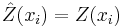$\hat{Z}(x_i)=Z(x_i)$ (assuming no measurement error is incurred)
The kriging estimation is the best linear unbiased estimator of if the assumptions hold. However (e.g. Cressie 1993):
- As with any method: If the assumptions do not hold, kriging might be bad.
- There might be better nonlinear and/or biased methods.
- No properties are guaranteed, when the wrong variogram is used. However typically still a 'good' interpolation is achieved.
- Best is not necessarily good: e.g. In case of no spatial dependence the kriging interpolation is only as good as the arithmetic mean.
Kriging provides $\sigma_k^2$ as a measure of precision. However this measure relies on the correctness of the variogram.

Related terms and techniques

Terms

A series of related terms were also named after Krige, including kriged estimate, kriged estimator, kriging variance, kriging covariance, zero kriging variance, unity kriging covariance, kriging matrix, kriging method, kriging model, kriging plan, kriging process, kriging system, block kriging, co-kriging, disjunctive kriging, linear kriging, ordinary kriging, point kriging, random kriging, regular grid kriging, simple kriging and universal kriging.

Related methods

Kriging is mathematically closely related to regression analysis. Both theories derive a best linear unbiased estimator, based on assumptions on covariances, make use of Gauss-Markov theorem to prove independence of the estimate and error, and make use of very similar formulae. They are nevertheless useful in different frameworks: kriging is made for interpolation of a single realisation of a random field, while regression models are based on multiple observations of a multivariate dataset.

In the statistical community the same technique is also known as Gaussian process regression, Kolmogorov Wiener prediction, or best linear unbiased prediction.

The kriging interpolation may also be seen as a spline in a reproducing kernel Hilbert space, with reproducing kernel given by the covariance function.^[12] The difference with the classical kriging approach is provided by the interpretation: while the spline is motivated by a minimum norm interpolation based on a Hilbert space structure, kriging is motivated by an expected squared prediction error based on a stochastic model.

Kriging with polynomial trend surfaces is mathematically identical to generalized least squares polynomial curve fitting.

Kriging can also be understood as a form of Bayesian inference.^[13] Kriging starts with a prior distribution over functions. This prior takes the form of a Gaussian process: $N$ samples from a function will be normally distributed, where the covariance between any two samples is the covariance function (or kernel) of the Gaussian process evaluated at the spatial location of two points. A set of values is then observed, each value associated with a spatial location. Now, a new value can be predicted at any new spatial location, by combining the Gaussian prior with a Gaussian likelihood function for each of the observed values. The resulting posterior distribution is also Gaussian, with a mean and covariance that can be simply computed from the observed values, their variance, and the kernel matrix derived from the prior.

History

The theory of kriging was developed by the French mathematician Georges Matheron based on the Master's thesis of Daniel Gerhardus Krige, the pioneering plotter of distance-weighted average gold grades at the Witwatersrand reef complex. The English verb is to krige and the most common adjective is kriging. The method was called krigeage for the first time in Matheron's 1960 Krigeage d'un Panneau Rectangulaire par sa Périphérie. Matheron, in this Note Géostatistique No 28, derives k*, his estimateur and a precursor to the kriged estimate or kriged estimator. In classical statistics, Matheron's k* is the length-weighted average grade of each of his panneaux in his set. What Matheron failed to derive was var(k*), the variance of his estimateur. On the contrary, he computed the length-weighted average grade of each panneau but did not compute the variance of its central value. In time, he replaced length-weighted average grades for three-dimensional sample spaces such as Matheronian blocks of ore with more abundant distance-weighted average grades for zero-dimensional sample spaces such as Matheronian points.

References

^ Sacks, J. and Welch, W.~J. and Mitchell, T.~J. and Wynn, H.~P. (1989). Design and Analysis of Computer Experiments. 4. Statistical Science. pp. 409–435.
^ Hanefi Bayraktar and F. Sezer. Turalioglu (2005) A Kriging-based approach for locating a sampling site—in the assessment of air quality, SERRA, v.19, n.4, DOI 10.1007/s00477-005-0234-8, p. 301-305
^ Chiles, J.-P. and P. Delfiner (1999) Geostatistics, Modeling Spatial uncertainty, Wiley Series in Probability and statistics.
^ Zimmerman, D.A. et al. (1998) A comparison of seven geostatistically based inverse approaches to estimate transmissivies for modelling advective transport by groundwater flow, Water Resource. Res., v.34, n.6, p.1273-1413
^ Tonkin M.J. Larson (2002) Kriging Water Levels with a Regional-Linear and Point Logarithmic Drift, Ground Water, v. 33, no 1., p. 338-353,
^ Journel, A.G. and C.J. Huijbregts (1978) Mining Geostatistics, Academic Press London
^ Andrew Richmond (2003) Financially Efficient Ore Selection Incorporating Grade Uncertainty, Mathematical Geology, v. 35, n.2, pp. 195-215
^ Goovaerts (1997) Geostatistics for natural resource evaluation,
^ X. Emery (2005) Simple and Ordinary Kriging Multigaussian Kriging for Estimating recovevearble Reserves, Mathematical Geology, v. 37, n. 3, pp. 295-319)
^ A. Stein, F. van der Meer, B. Gorte (Eds.) (2002) Spatial Statistics for remote sensing
^ Barris, J. (2008) An expert system for appraisal by the method of comparison. PhD Thesis, UPC, Barcelona
^ Grace Wahba (1990). Spline Models for Observational Data. 59. SIAM. pp. 162.
^ Williams, Christopher K.I. (1998). "Prediction with Gaussian processes: From linear regression to linear prediction and beyond". In M. I. Jordan. Learning in graphical models. MIT Press. pp. 599–612.

Books

Abramowitz, M., and Stegun, I. (1972), Handbook of Mathematical Functions, Dover Publications, New York.
Banerjee, S., Carlin, B.P. and Gelfand, A.E. (2004). Hierarchical Modeling and Analysis for Spatial Data. Chapman and Hall/CRC Press, Taylor and Francis Group.
Chiles, J.-P. and P. Delfiner (1999) Geostatistics, Modeling Spatial uncertainty, Wiley Series in Probability and statistics.
Cressie, N (1993) Statistics for spatial data, Wiley, New York
David, M (1988) Handbook of Applied Advanced Geostatistical Ore Reserve Estimation, Elsevier Scientific Publishing
Deutsch, C.V., and Journel, A. G. (1992), GSLIB - Geostatistical Software Library and User's Guide, Oxford University Press, New York, 338 pp.
Goovaerts, P. (1997) Geostatistics for Natural Resources Evaluation, Oxford University Press, New York
Isaaks, E. H., and Srivastava, R. M. (1989), An Introduction to Applied Geostatistics, Oxford University Press, New York, 561 pp.
Journel, A. G. and C. J. Huijbregts (1978) Mining Geostatistics, Academic Press London
Journel, A. G. (1989), Fundamentals of Geostatistics in Five Lessons, American Geophysical Union, Washington D.C.
Press, WH; Teukolsky, SA; Vetterling, WT; Flannery, BP (2007), "Section 3.7.4. Interpolation by Kriging", Numerical Recipes: The Art of Scientific Computing (3rd ed.), New York: Cambridge University Press, ISBN 978-0-521-88068-8, http://apps.nrbook.com/empanel/index.html?pg=144 . Also, "Section 15.9. Gaussian Process Regression".
Stein, M. L. (1999), Statistical Interpolation of Spatial Data: Some Theory for Kriging, Springer, New York.
Wackernagel, H. (1995) Multivariate Geostatistics - An Introduction with Applications, Springer Berlin

Historical references

Agterberg, F P, Geomathematics, Mathematical Background and Geo-Science Applications, Elsevier Scientific Publishing Company, Amsterdam, 1974
Cressie, N. A. C., The Origins of Kriging, Mathematical Geology, v. 22, pp 239–252, 1990
Krige, D.G, A statistical approach to some mine valuations and allied problems at the Witwatersrand, Master's thesis of the University of Witwatersrand, 1951
Link, R F and Koch, G S, Experimental Designs and Trend-Surface Analsysis, Geostatistics, A colloquium, Plenum Press, New York, 1970
Matheron, G., "Principles of geostatistics", Economic Geology, 58, pp 1246–1266, 1963
Matheron, G., "The intrinsic random functions, and their applications", Adv. Appl. Prob., 5, pp 439–468, 1973
Merriam, D F, Editor, Geostatistics, a colloquium, Plenum Press, New York, 1970